Galaxy Simulator Parameters Defined

Quick Links to Specific Definitions

Potential Solver Methods:
Potential Types:
Integration Methods:
Other Simulator Parameters

Potential Solver Methods
The simulator uses potentials of the form Φ_total = Φ_bg+ Φ_sg to derive the force on the particles, where Φ_bg is an imposed background potential and Φ_sg is the potential due to the self-gravity of the particles. Self-gravity can be turned on or off (as can the background potential) and integrated by selecting the desired potential solver method.

No Self Gravity: This option turns off self-gravity so particle motion may be evaluated using only a background potential.

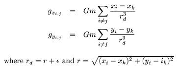
Direct Force Summation: This method finds the acceleration on each particle directly by adding up the accelerations due to all the other particles individually according to

This is a very inefficient and costly integration method; it should only be used when evaluating a small number of particles.

Fourier Method: The potential can be found more efficiently using the Fourier method. This method uses Fourier transforms on a grid of N_x x N_y cells to determine the potential and mass density in each cell. The complete method is complicated, but is much more efficient for determining the potential due to a large number of bodies and should be used instead of direct force summation unless only a small number of particles are involved. For a more complete description of this method see the paper written by the original authors of the simulator.

Potential Types
The force, and therefore the acceleration, experienced by a particle is derived from the potential field in which the particle resides: F = -∇Φ. The simulator provides many models for the background potential.

No Background Potential: This option turns off the background potential so that particle trajectories may be evolved using only self-gravity.

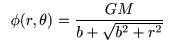
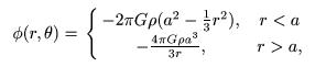
Power Law Potential: The simulator uses a power law potential of the form

,
where ε is a smoothing parameter and is input as param2; the value of n is given by param1. n = 1 provides a Keplerian potential.

Time Dependent Bar Potential: The time dependent and independent bar potentials used by the simulator are logarithmic potentials of the form

The variable ε is a parameter which scales the effect of the bar and is input as param1. Ω is the angular frequency and is given by param2.

Harmonic Potential: This option is a harmonic potential is of the form

In the simulator, the scaling factors A and B are input as param1 = A and param2 = B. These scaling factors determine the relative strength of the field in x and y.

Isochrone Potential: The isochrone potential is a reasonable approximation to a disc galaxy with roughly constant density near the center and the density going to zero at larger radii. The simulator uses the form

The variable b is given by param1 and the disc mass M is param2.

Homogeneous Sphere Potential: The homogeneous sphere simulates the potential due to a sphere of uniform density. This is a practical approximation to a large massive central object or the potential due to a halo near the center of an otherwise thin disc galaxy. The form used is
Homogeneous
Sphere Potential

The sphere radius a is input as param1, and the sphere density ρ is param2.

"Galaxy" Potential: The galaxy potential is actually a combination of Keplerian, homogeneous sphere and logarithmic potentials as described above. This combination is designed to model a large disc galaxy with a halo and central compact object. For this potential the input parameters param1 and param2 are not used.

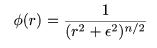Integration Methods
Finding each particle's position and velocity for each timestep requires knowing the particle's acceleration and initial conditions for that timestep. The acceleration is determined using the potential at each location according to

,
and similarly for the y direction, noting that the simulator normalizes all particle masses to unity. From there, the positions and velocities are found using one of the available numerical integration schemes. For in-depth detail of these methods, with computer code, see W.H. Press, S.A. Teukolsky, W.T. Vetterling, and B.P. Flannery, Numerical Recipes in C: The Art of Scientific Computing, 2nd edition, 1997. Additionally, the graphical representations of the integration methods were obtained from http://www.physics.drexel.edu/courses/CompPhys/Integrators/ prepeared by Steve McMillan at Drexel University.

Euler Method: The Euler integration scheme is the simplest available in the simulator. It is computationally cheap, but because it is only first order its error term is second order in the timestep, making it a relatively inaccurate integration method. A graphical representation along with the formulae is shown below.

Euler Integration Method

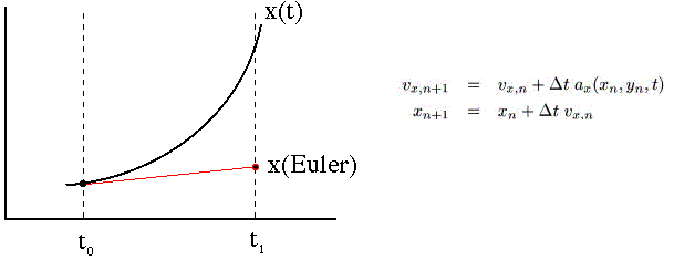
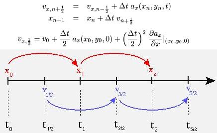
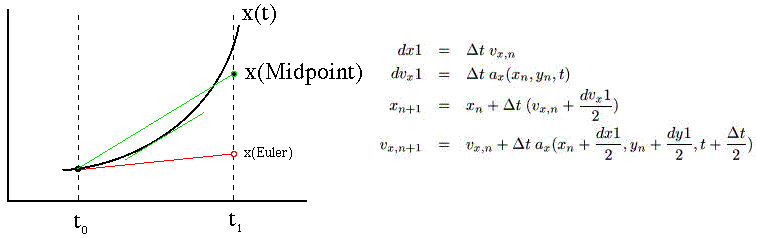
Leapfrog Method: The Leapfrog integration method is only slightly higher in computational cost than the Euler method, but it's error term is third order. As can be seen in the diagram and formulae, this method uses the derivatives at the midpoint of each step. This only requires one additional step to be taken in order to move the velocity a half step ahead of the position. Because of its better accuracy while still keeping the simulation generation time relatively low the Leapfrog method is the default integration scheme.

Midpoint Method: The Midpoint method is similar to the Euler method in that it starts by taking an Euler "trial step." It then uses the values obtained by the trial step to take real steps according to the formulae shown. This method also has an error term that is third order, but it is more computationally expensive than the Leapfrog method. It is important, however, since it is more easily generalized to the much more accurate (and expensive) Runge-Kutta and Cash-Karp schemes.

Midpoint Integration Method

Runge-Kutta Method: The Runge-Kutta method is a fourth order integration technique similar to an expanded Midpoint scheme. This method takes four trial steps and uses their weighted average to advance the particle according to the formulae shown below. It is highly accurate, having a fifth order error term, but it is computationally expensive.

4th Order Runge-Kutta Integration Method

4th Order Runge-Kutta Integration Method

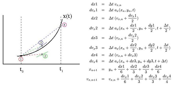
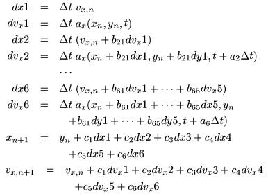
Cash-Karp Method: The Cash-Karp method is basically the same as a fifth order Runge-Kutta scheme. It uses various constants found by Cash and Karp (see Numerical Recipes, 2nd edition) in the formulae shown. This is the most accurate integration technique available on the simulator, having a sixth order error term, but it is less practicle because of its enormously high cost in computational time.

Self Gravity Leapfrog Method:

Other Simulator Parameters

Time Duration: This input gives the total time duration of the simulation.

Timestep: The timestep sets the time interval Δt used in the integration scheme.

Image Frequency: The image frequency tells the simulator how often to "dump" the simulation data in numbers of timesteps. Each of these dumps is used to create a frame in the final movie, so the number of frames that will be present is given by the time duration divided by the product of the timestep and image frequency.

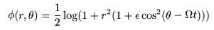
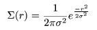
Alpha: The parameter "Alpha" is a measure of dispersion in a Gaussian surface density distribution. The simulator uses a surface density of the form

Alpha provides the value of the variable σ in the above formula.

Other Stuff

Students working on the simulators available in the Digital Demo Room participate in the "Research Experience for Undergraduates", or REU, program in the Physics Department of the University of Illinois. The students give presentations on their projects and also write a scientific paper. The paper for the Thin Disc Galaxy simulator, which was built by Scott Olsson and Geert Vrijsen during the 2001 REU program, is available here for anyone interested in seeing the development of this pedagogical project.

Return to the simulator!